library(MASS)chapter 6, chapter 7
data(Boston)head(Boston)| crim | zn | indus | chas | nox | rm | age | dis | rad | tax | ptratio | black | lstat | medv | |
|---|---|---|---|---|---|---|---|---|---|---|---|---|---|---|
| <dbl> | <dbl> | <dbl> | <int> | <dbl> | <dbl> | <dbl> | <dbl> | <int> | <dbl> | <dbl> | <dbl> | <dbl> | <dbl> | |
| 1 | 0.00632 | 18 | 2.31 | 0 | 0.538 | 6.575 | 65.2 | 4.0900 | 1 | 296 | 15.3 | 396.90 | 4.98 | 24.0 |
| 2 | 0.02731 | 0 | 7.07 | 0 | 0.469 | 6.421 | 78.9 | 4.9671 | 2 | 242 | 17.8 | 396.90 | 9.14 | 21.6 |
| 3 | 0.02729 | 0 | 7.07 | 0 | 0.469 | 7.185 | 61.1 | 4.9671 | 2 | 242 | 17.8 | 392.83 | 4.03 | 34.7 |
| 4 | 0.03237 | 0 | 2.18 | 0 | 0.458 | 6.998 | 45.8 | 6.0622 | 3 | 222 | 18.7 | 394.63 | 2.94 | 33.4 |
| 5 | 0.06905 | 0 | 2.18 | 0 | 0.458 | 7.147 | 54.2 | 6.0622 | 3 | 222 | 18.7 | 396.90 | 5.33 | 36.2 |
| 6 | 0.02985 | 0 | 2.18 | 0 | 0.458 | 6.430 | 58.7 | 6.0622 | 3 | 222 | 18.7 | 394.12 | 5.21 | 28.7 |
nrow(Boston)
506
보스턴 집값 데이터 이 데이터는 보스턴 근교 지역의 집값 및 다른 정보를 포함한다.
MASS 패키지를 설치하면 데이터를 로딩할 수 있다.
B보스턴 근교 506개 지역에 대한 범죄율 (crim)등 14개의 변수로 구성
• crim : 범죄율
• zn: 25,000평방비트 기준 거지주 비율
• indus: 비소매업종 점유 구역 비율
• chas: 찰스강 인접 여부 (1=인접, 0=비인접)
• nox: 일산화질소 농도 (천만개 당)
• rm: 거주지의 평균 방 갯수 ***
• age: 1940년 이전에 건축된 주택의 비율
• dis: 보스턴 5대 사업지구와의 거리
• rad: 고속도로 진입용이성 정도
• tax: 재산세율 (10,000달러 당)
• ptratio: 학생 대 교사 비율
• black: 1000(B − 0.63)2, B: 아프리카계 미국인 비율
• lstat : 저소득층 비율 ****
• medv: 주택가격의 중앙값 (단위:1,000달러 당)
데이터 세 변수만 가지고 산점도 그려보기
음의 상관관계가 있는 것 같기도 하고~
pairs(Boston[,which(names(Boston) %in% c('medv', 'rm', 'lstat'))], pch=16, col='darkorange')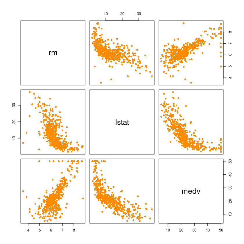
- lm(y ~ x_1 + x_2, data)
fit_Boston<-lm(medv~rm+lstat, data=Boston)F-statistic: 444.3 on 2 and 503 DF, p-value: < 2.2e-16R-squared: 0.6386- 집값 y의 총변동 중에 회귀모형이 63.86%정도 설명하고 있다.
Adjusted R-squared: 0.6371- 설명변수가 증가하면 R-squared값이 증가하는 현상때문에 수정된 R-squared값이 필요
- 모형 비교시 Adjusted R-squared가 나을 수도 있음
- rm,lstat의 p-value
<2e-16
summary(fit_Boston)
Call:
lm(formula = medv ~ rm + lstat, data = Boston)

Residuals:
    Min      1Q  Median      3Q     Max
-18.076  -3.516  -1.010   1.909  28.131

Coefficients:
            Estimate Std. Error t value Pr(>|t|)
(Intercept) -1.35827    3.17283  -0.428    0.669
rm           5.09479    0.44447  11.463   <2e-16 ***
lstat       -0.64236    0.04373 -14.689   <2e-16 ***
---
Signif. codes:  0 ‘***’ 0.001 ‘**’ 0.01 ‘*’ 0.05 ‘.’ 0.1 ‘ ’ 1

Residual standard error: 5.54 on 503 degrees of freedom
Multiple R-squared:  0.6386,    Adjusted R-squared:  0.6371
F-statistic: 444.3 on 2 and 503 DF, p-value: < 2.2e-16- 원하는 변수만 추출해내서 회귀분석 진행가능
dt <- Boston[,which(names(Boston) %in% c('medv', 'rm', 'lstat'))]head(dt)| rm | lstat | medv | |
|---|---|---|---|
| <dbl> | <dbl> | <dbl> | |
| 1 | 6.575 | 4.98 | 24.0 |
| 2 | 6.421 | 9.14 | 21.6 |
| 3 | 7.185 | 4.03 | 34.7 |
| 4 | 6.998 | 2.94 | 33.4 |
| 5 | 7.147 | 5.33 | 36.2 |
| 6 | 6.430 | 5.21 | 28.7 |
.쓰면 설명변수 다 쓰겠다는 의미
fit_Boston<-lm(medv~., data=dt)\(\hat{y} = -1.3583 + 5.0948*rm - 0.6424*lstat\)
저소득층이 변하지 않고 방이 하나 더 증가한다면 집값의 중앙값은 5.0948 정도 증가한다.
방의 수는 변하지 않고 저소득층이 증가한다면 집값의 중앙값은 0.6424 정도 감소한다.
SSR = 41308.84 = 20654.42 + 20654.42
밑의 F 통계량이 아니라 summary 의 F 통계량을 봐야 한다.
anova(fit_Boston)| Df | Sum Sq | Mean Sq | F value | Pr(>F) | |
|---|---|---|---|---|---|
| <int> | <dbl> | <dbl> | <dbl> | <dbl> | |
| rm | 1 | 20654.42 | 20654.41622 | 672.9039 | 8.266887e-95 |
| lstat | 1 | 6622.57 | 6622.56999 | 215.7579 | 6.669365e-41 |
| Residuals | 503 | 15439.31 | 30.69445 | NA | NA |
\(var(\hat{\beta}) = (X^TX)^{-1} \sigma^2\)
vcov(fit_Boston) | (Intercept) | rm | lstat | |
|---|---|---|---|
| (Intercept) | 10.06683612 | -1.39248641 | -0.099178133 |
| rm | -1.39248641 | 0.19754958 | 0.011930670 |
| lstat | -0.09917813 | 0.01193067 | 0.001912441 |
confint(fit_Boston, level = 0.95)| 2.5 % | 97.5 % | |
|---|---|---|
| (Intercept) | -7.5919003 | 4.8753547 |
| rm | 4.2215504 | 5.9680255 |
| lstat | -0.7282772 | -0.5564395 |
coef(fit_Boston) + qt(0.975, 503) * summary(fit_Boston)$coef[,2]- (Intercept)
- 4.87535465808389
- rm
- 5.96802553290791
- lstat
- -0.556439501179164
coef(fit_Boston) - qt(0.975, 503) * summary(fit_Boston)$coef[,2]- (Intercept)
- -7.59190028183298
- rm
- 4.22155043576519
- lstat
- -0.728277167309095
평균반응, 개별 y 추정
\(E(Y|x_0), y = E(Y|x_0) + \epsilon\)
new_dt <- data.frame(rm=7, lstat=10)\(\hat{y}_0 = -1.3583 + 5.0948*7 - 0.6424*10\)
predict(fit_Boston, newdata = new_dt)
1: 27.88165973604
평균반응
predict(fit_Boston,
        newdata = new_dt,
        interval = c("confidence"),
level = 0.95) | fit | lwr | upr | |
|---|---|---|---|
| 1 | 27.88166 | 27.17347 | 28.58985 |
개별 y
predict(fit_Boston, newdata = new_dt,
        interval = c("prediction"),
level = 0.95) | fit | lwr | upr | |
|---|---|---|---|
| 1 | 27.88166 | 16.97375 | 38.78957 |
- fit은 같고 lwr,upr만 달라진다.
잔차분석
\(\epsilon\) : 선형성, 등분산성, 정규성, 독립성
yhat <- fitted_values(fit_Boston)yhat <- fitted(fit_Boston)res <- resid(fit_Boston)잔차그림 - 대칭 아니다 - u 턴 커브 모형이다. - 애초에 산점도에서도 커브가 보였다. - 나중에 제곱텀 넣어볼 예정
plot(res ~ yhat,pch=16, ylab = 'Residual')
abline(h=0, lty=2, col='grey')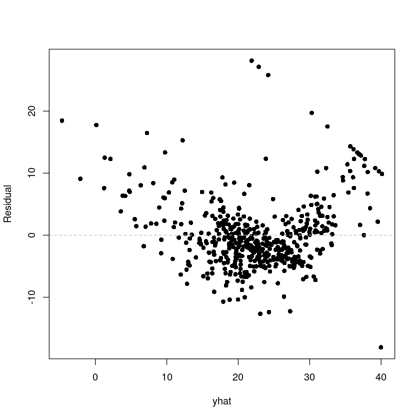
- 제곱텀 필요해보인다.
plot(res ~ dt$rm,pch=16, ylab = 'Residual')
abline(h=0, lty=2, col='grey')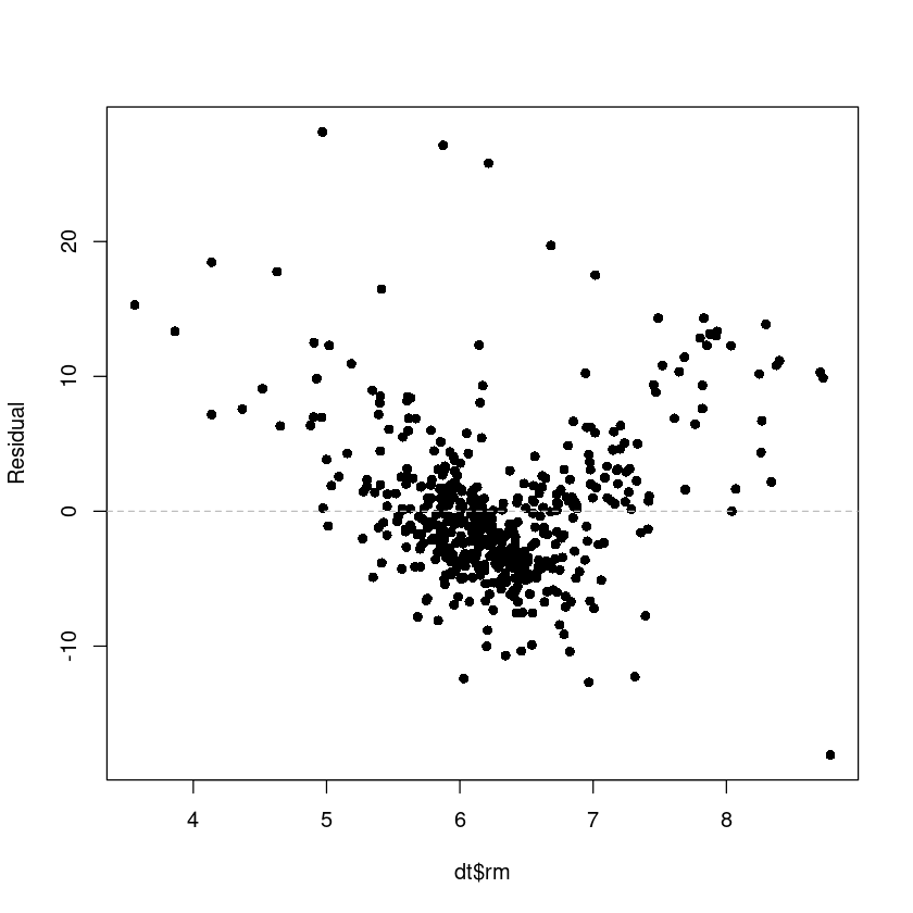
- 제곱텀 필요해보인다.
plot(res ~ dt$lstat,pch=16, ylab = 'Residual')
abline(h=0, lty=2, col='grey')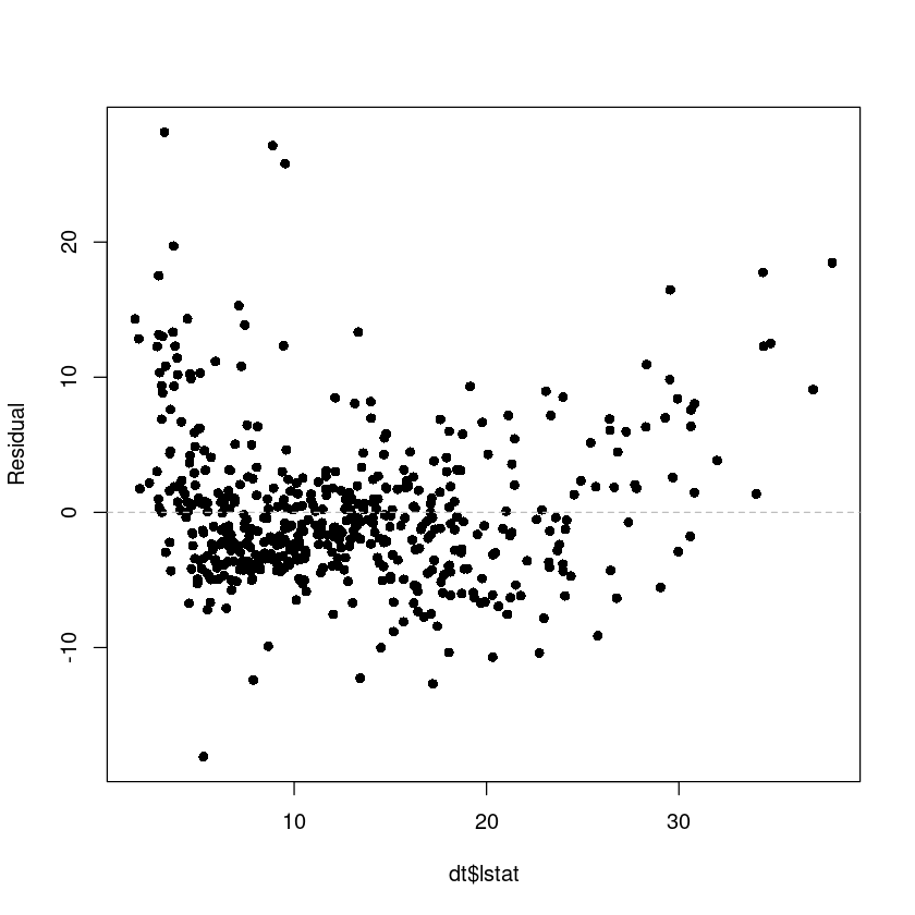
독립성검정 : DW test
library(lmtest)\(H_0 : \text{ uncorrelated vs } H_1 : \rho \neq 0\)
dwtest(fit_Boston, alternative = "two.sided")
    Durbin-Watson test

data:  fit_Boston
DW = 0.83421, p-value < 2.2e-16
alternative hypothesis: true autocorrelation is not 0- p-value < 2.2e-16로 귀무가설 기각한다. 잔차는 독립이 아니다.
잔차의 QQ plot
정규성 확인 결과도 좋지 않음
qqnorm(res, pch=16)
qqline(res, col = 2)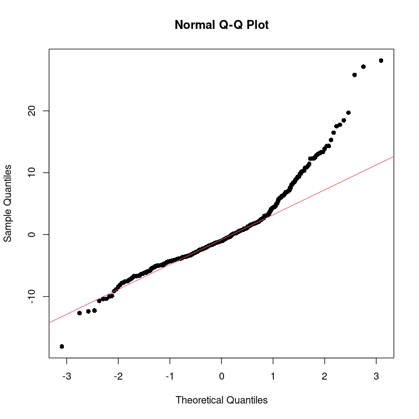
head(dt)| rm | lstat | medv | |
|---|---|---|---|
| <dbl> | <dbl> | <dbl> | |
| 1 | 6.575 | 4.98 | 24.0 |
| 2 | 6.421 | 9.14 | 21.6 |
| 3 | 7.185 | 4.03 | 34.7 |
| 4 | 6.998 | 2.94 | 33.4 |
| 5 | 7.147 | 5.33 | 36.2 |
| 6 | 6.430 | 5.21 | 28.7 |
dt$lstat2 <- (dt$lstat)^2head(dt)| rm | lstat | medv | lstat2 | |
|---|---|---|---|---|
| <dbl> | <dbl> | <dbl> | <dbl> | |
| 1 | 6.575 | 4.98 | 24.0 | 24.8004 |
| 2 | 6.421 | 9.14 | 21.6 | 83.5396 |
| 3 | 7.185 | 4.03 | 34.7 | 16.2409 |
| 4 | 6.998 | 2.94 | 33.4 | 8.6436 |
| 5 | 7.147 | 5.33 | 36.2 | 28.4089 |
| 6 | 6.430 | 5.21 | 28.7 | 27.1441 |
1번 방법
fit_Boston2<-lm(medv~., data=dt)# 이렇게 쓰면 위에와 결과 같음
fit_Boston2<-lm(medv~rm+lstat+lstat^2, data=Boston)2번 방법 변수 생성 없이 수행가능
fit_Boston2<-lm(medv~rm+lstat+I(lstat^2), data=Boston)Adjusted R-squared: 0.7013이 63%에서 증가한 모습
summary(fit_Boston2)
Call:
lm(formula = medv ~ rm + lstat + I(lstat^2), data = Boston)

Residuals:
     Min       1Q   Median       3Q      Max
-18.1427  -3.2429  -0.4829   2.3607  27.0256

Coefficients:
            Estimate Std. Error t value Pr(>|t|)
(Intercept) 11.68964    3.13810   3.725 0.000217 ***
rm           4.22727    0.41172  10.267  < 2e-16 ***
lstat       -1.84863    0.12213 -15.136  < 2e-16 ***
I(lstat^2)   0.03634    0.00348  10.443  < 2e-16 ***
---
Signif. codes:  0 ‘***’ 0.001 ‘**’ 0.01 ‘*’ 0.05 ‘.’ 0.1 ‘ ’ 1

Residual standard error: 5.027 on 502 degrees of freedom
Multiple R-squared:  0.7031,    Adjusted R-squared:  0.7013
F-statistic: 396.2 on 3 and 502 DF,  p-value: < 2.2e-16
yhat2 <- fitted.values(fit_Boston2)res2 <- resid(fit_Boston2)- 곡선 느낌은 사라지고 outlier는 보이고 있다.
plot(res2 ~ yhat2,pch=16, ylab = 'Residual')
abline(h=0, lty=2, col='grey')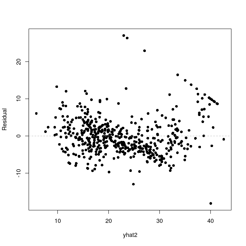
- 꼬리가 죽은 모습
qqnorm(res2, pch=16)
qqline(res2, col = 2)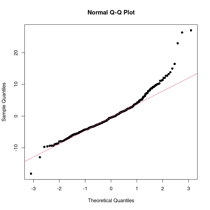
\(H_0 : \text{ uncorrelated vs } H_1 : \rho \neq 0\)
dwtest(fit_Boston2, alternative = "two.sided")
    Durbin-Watson test

data:  fit_Boston2
DW = 0.84831, p-value < 2.2e-16
alternative hypothesis: true autocorrelation is not 0- 여전히 잔차가 독립이 아니고 기각한다.
fit_Boston3 <- lm(medv~rm, data=Boston)fit_Boston4 <- lm(medv~lstat, data=Boston)summary(fit_Boston3)
Call:
lm(formula = medv ~ rm, data = Boston)

Residuals:
    Min      1Q  Median      3Q     Max
-23.346  -2.547   0.090   2.986  39.433

Coefficients:
            Estimate Std. Error t value Pr(>|t|)
(Intercept)  -34.671      2.650  -13.08   <2e-16 ***
rm             9.102      0.419   21.72   <2e-16 ***
---
Signif. codes:  0 ‘***’ 0.001 ‘**’ 0.01 ‘*’ 0.05 ‘.’ 0.1 ‘ ’ 1

Residual standard error: 6.616 on 504 degrees of freedom
Multiple R-squared:  0.4835,    Adjusted R-squared:  0.4825
F-statistic: 471.8 on 1 and 504 DF, p-value: < 2.2e-16summary(fit_Boston4)
Call:
lm(formula = medv ~ lstat, data = Boston)

Residuals:
    Min      1Q  Median      3Q     Max
-15.168  -3.990  -1.318   2.034  24.500

Coefficients:
            Estimate Std. Error t value Pr(>|t|)
(Intercept) 34.55384    0.56263   61.41   <2e-16 ***
lstat       -0.95005    0.03873  -24.53   <2e-16 ***
---
Signif. codes:  0 ‘***’ 0.001 ‘**’ 0.01 ‘*’ 0.05 ‘.’ 0.1 ‘ ’ 1

Residual standard error: 6.216 on 504 degrees of freedom
Multiple R-squared:  0.5441,    Adjusted R-squared:  0.5432
F-statistic: 601.6 on 1 and 504 DF, p-value: < 2.2e-16x1<-c(4,8,9,8,8,12,6,10,6,9)
x2<-c(4,10,8,5,10,15,8,13,5,12)
y<-c(9,20,22,15,17,30,18,25,10,20)FM
fit<-lm(y~x1+x2)summary(fit)
Call:
lm(formula = y ~ x1 + x2)

Residuals:
    Min      1Q  Median      3Q     Max
-2.4575 -1.9100  0.3314  0.6388  3.2628

Coefficients:
            Estimate Std. Error t value Pr(>|t|)
(Intercept)  -0.6507     2.9075  -0.224   0.8293
x1            1.5515     0.6462   2.401   0.0474 *
x2            0.7599     0.3968   1.915   0.0970 .
---
Signif. codes:  0 ‘***’ 0.001 ‘**’ 0.01 ‘*’ 0.05 ‘.’ 0.1 ‘ ’ 1

Residual standard error: 2.278 on 7 degrees of freedom
Multiple R-squared:  0.9014,    Adjusted R-squared:  0.8732
F-statistic: 32 on 2 and 7 DF, p-value: 0.0003011anova(fit)| Df | Sum Sq | Mean Sq | F value | Pr(>F) | |
|---|---|---|---|---|---|
| <int> | <dbl> | <dbl> | <dbl> | <dbl> | |
| x1 | 1 | 313.04348 | 313.043478 | 60.323103 | 0.0001100467 |
| x2 | 1 | 19.03040 | 19.030400 | 3.667135 | 0.0970444465 |
| Residuals | 7 | 36.32612 | 5.189446 | NA | NA |
install.packages("car")library(car)\(H_0 : T\times\beta = c\)
$b_1-b_2=0 (0,1,-1) $
\(H_0 : \beta_1 = \beta_2\)
linearHypothesis(fit, c(0,1,-1), 0)| Res.Df | RSS | Df | Sum of Sq | F | Pr(>F) | |
|---|---|---|---|---|---|---|
| <dbl> | <dbl> | <dbl> | <dbl> | <dbl> | <dbl> | |
| 1 | 8 | 39.53514 | NA | NA | NA | NA |
| 2 | 7 | 36.32612 | 1 | 3.209014 | 0.6183731 | 0.4574425 |
- 제약조건, T matrix c(0,1,-1)
- c = 0
3.209014 / (36.32612/7)
0.618373170600108
같다~
\(H_0 : \beta_1 = 1\)
linearHypothesis(fit, c(0,1,0), 1)| Res.Df | RSS | Df | Sum of Sq | F | Pr(>F) | |
|---|---|---|---|---|---|---|
| <dbl> | <dbl> | <dbl> | <dbl> | <dbl> | <dbl> | |
| 1 | 8 | 40.10492 | NA | NA | NA | NA |
| 2 | 7 | 36.32612 | 1 | 3.778797 | 0.7281696 | 0.4217136 |
- 기각하지 못함
\(H_0 : \beta_1 = \beta_2 + 1\)
linearHypothesis(fit, c(0,1,-1), 1)| Res.Df | RSS | Df | Sum of Sq | F | Pr(>F) | |
|---|---|---|---|---|---|---|
| <dbl> | <dbl> | <dbl> | <dbl> | <dbl> | <dbl> | |
| 1 | 8 | 36.54865 | NA | NA | NA | NA |
| 2 | 7 | 36.32612 | 1 | 0.2225273 | 0.04288074 | 0.841845 |
F0
0.0428807391894599
\(H_0 : \beta_1 = \beta_2 + 1\)
\(y = b_0 + b_1x_1 + b_2x_2 + \epsilon = b_0+x_1 + b_2(x_1+x_2)+\epsilon\)
\(y-x_1 = b_0+b_2(x_1+x_2)+\epsilon\) : RM
y1 <- y-x1
z1 <- x1 + x2
fit2 <- lm(y1~z1)summary(fit2)
Call:
lm(formula = y1 ~ z1)

Residuals:
    Min      1Q  Median      3Q     Max
-2.5054 -1.9294  0.4236  0.6821  3.4473

Coefficients:
            Estimate Std. Error t value Pr(>|t|)
(Intercept)  -1.0014     2.2175  -0.452 0.663574
z1            0.6824     0.1242   5.493 0.000578 ***
---
Signif. codes:  0 ‘***’ 0.001 ‘**’ 0.01 ‘*’ 0.05 ‘.’ 0.1 ‘ ’ 1

Residual standard error: 2.137 on 8 degrees of freedom
Multiple R-squared:  0.7904,    Adjusted R-squared:  0.7642
F-statistic: 30.17 on 1 and 8 DF, p-value: 0.0005785anova(fit2)| Df | Sum Sq | Mean Sq | F value | Pr(>F) | |
|---|---|---|---|---|---|
| <int> | <dbl> | <dbl> | <dbl> | <dbl> | |
| z1 | 1 | 137.85135 | 137.851351 | 30.17378 | 0.0005784583 |
| Residuals | 8 | 36.54865 | 4.568581 | NA | NA |
FM
anova(fit) | Df | Sum Sq | Mean Sq | F value | Pr(>F) | |
|---|---|---|---|---|---|
| <int> | <dbl> | <dbl> | <dbl> | <dbl> | |
| x1 | 1 | 313.04348 | 313.043478 | 60.323103 | 0.0001100467 |
| x2 | 1 | 19.03040 | 19.030400 | 3.667135 | 0.0970444465 |
| Residuals | 7 | 36.32612 | 5.189446 | NA | NA |
RM
anova(fit2) | Df | Sum Sq | Mean Sq | F value | Pr(>F) | |
|---|---|---|---|---|---|
| <int> | <dbl> | <dbl> | <dbl> | <dbl> | |
| z1 | 1 | 137.85135 | 137.851351 | 30.17378 | 0.0005784583 |
| Residuals | 8 | 36.54865 | 4.568581 | NA | NA |
\(F = {(SSE_RM - SSE_FM)/r} / {SSE_FM/(n-p-1)}\)
SSE_FM
SSE_FM <- anova(fit)$Sum[3] SSE_RM
SSE_RM <- anova(fit2)$Sum[2] F0 <- (SSE_RM-SSE_FM)/(SSE_FM/7)
F0
0.0428807391894599
기각역 \(F_{0.05}(1,7)\)
qf(0.95, 1, 7)
5.59144785122073
기각할 수 없다.\(\beta_1\)은 \(\beta_2\)에 1 더한 값과 같다.